Key Considerations for Non-Expert Users
This page explains the main decisions needed to run and interpret the Vegetation Disturbance Occurrence tool.
The method uses a spectral trajectory break detection workflow. In practical terms, your main decisions are:
- Which spectral index and compositing period to use.
- Which analysis period to evaluate.
- Which segmentation threshold to use.
- How to convert continuous metrics into disturbance classes.
- How to validate and interpret the outputs.
You do not need to be a remote sensing specialist to start. Begin with a simple baseline setup, validate against known locations, and refine settings iteratively.
1. Choosing the Input Time Series
1.1 Use consistent seasonal composites
The tool is most stable when each year is represented by a composite of a comparable seasonal window (for example peak vegetation months). This reduces potential for false disturbance signals caused by seasonal mismatch.
Recommended practice:
- Focus on high-quality cloud-masked composites, and if necessary adjust BAP composite input parameters to achieve a cloud-free composite.
- Keep compositing logic unchanged across years and use the same input months for the composite every year.
1.2 Choose a spectral index that matches your objective
Common options:
- NBR: often strong for disturbance and woody vegetation change.
- SAVI: useful where exposed soil is frequent.
- NDVI: useful for broad greenness trends, but can saturate in dense vegetation.
If possible, test multiple indices to compare whether identified disturbance areas are consistent.
2. Choosing the Analysis Period
The algorithm expects a yearly sequence between a start year and end year. Choose a period long enough to capture:
- pre-disturbance baseline behavior,
- disturbance phase,
- and post-disturbance behavior.
As a practical minimum, the process requires a minimum of two years of data prior to the year of disturbance detection (a total of three years). A longer period generally improves the temporal segment/trajectory building.
3. Choosing the Segmentation Threshold
In the current implementation, the threshold controls when neighboring segments stop being merged (based on merge SSE). This is a complexity control, not a disturbance/no-disturbance threshold.
3.1 How threshold affects results
- Lower threshold: fewer merges, more segments, higher sensitivity to small trajectory changes.
- Higher threshold: more merges, fewer segments, smoother trajectories, lower sensitivity.
3.2 Practical tuning workflow
- Start with default threshold used by the tool configuration.
- Run a small test area with known disturbance examples.
- Compare outputs with a lower and higher threshold.
- Select the value that best balances omission and false positives.
4. Data Quality Rules
The disturbance detection code assumes clean numerical time series per pixel.
Critical rules:
- Missing values must be removed or masked before running the algorithm.
- Residual cloud and shadow contamination can create false disturbance detection.
- Sensor harmonization and consistent preprocessing are important in multi-year analyses.
If data quality is inconsistent, prioritize improving preprocessing before adjusting algorithm thresholds.
5. Interpreting the Outputs
The tool outputs continuous change metrics. The most important fields for disturbance occurrence mapping are:
- ChgYr: year of dominant disturbance segment.
- ChgMag: magnitude of dominant disturbance.
- ChgDur: duration of dominant disturbance segment.
- ChgEvl: rate of change (slope) during disturbance segment.
Additional fields (PreChg and PstChg) help interpret trajectory context before and after disturbance.
5.1 From metrics to categorical disturbance maps
Most users will apply thresholds to continuous metrics to classify disturbance occurrence.
Typical logic:
- Require disturbance magnitude beyond a chosen threshold.
- Optionally constrain disturbance year to a target monitoring period.
- Optionally constrain duration to remove very short noisy events.
- Optionally apply a minimum mapping unit so isolated patches below a chosen size are dropped.
Thresholds must be calibrated to landscape type and selected spectral index.
5.2 Worked example: disturbances in northern Democratic Republic of the Congo (DRC), 2023 to 2025
Start with a recent view of the landscape. The image below is the current ESRI Wayback basemap for an in the north of the Democratic Republic of the Congo (DRC). Bare soil, clearings, and tracks sit in and along the forest, so the landscape is visibly disturbed. The basemap does not say when each opening was made.
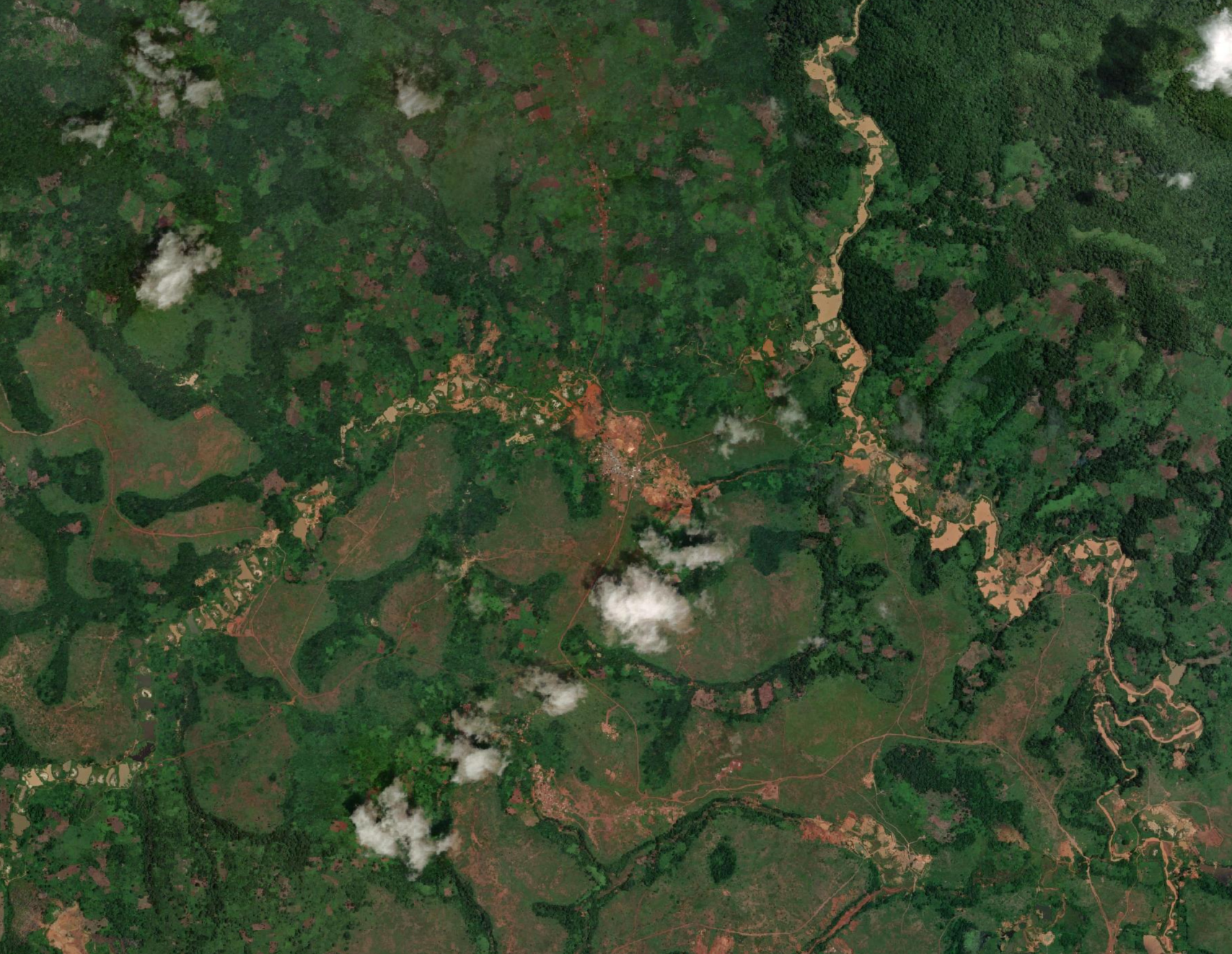
Current ESRI Wayback imagery for an area in northern DRC. Brown and tan patches are cleared or bare ground among forest. Clouds cover parts of the scene.
The Vegetation Disturbance Occurrence magnitude band (ChgMag) is a continuous measure of how large the spectral drop was. Threshold it to keep disturbances greater than a level you choose for the landscape and the spectral index. Pixels that pass that threshold still carry the disturbance year (ChgYr), so the same map shows both where a disturbance was large enough to keep and which year it occurred.
The map below is that step for a Vegetation Disturbance Occurrence run covering 2023 to 2025. Magnitude was already thresholded, and a minimum mapping unit of 7 pixels was applied, so patches smaller than that size are not drawn. Each color is one disturbance year in that window (Yellow = 2023, Light blue = 2024, Pink = 2025). Many of the kept patches follow the larger clearings on the basemap. Some of the other disturbances seen may have occurred outside of the 2023 to 2025 period.
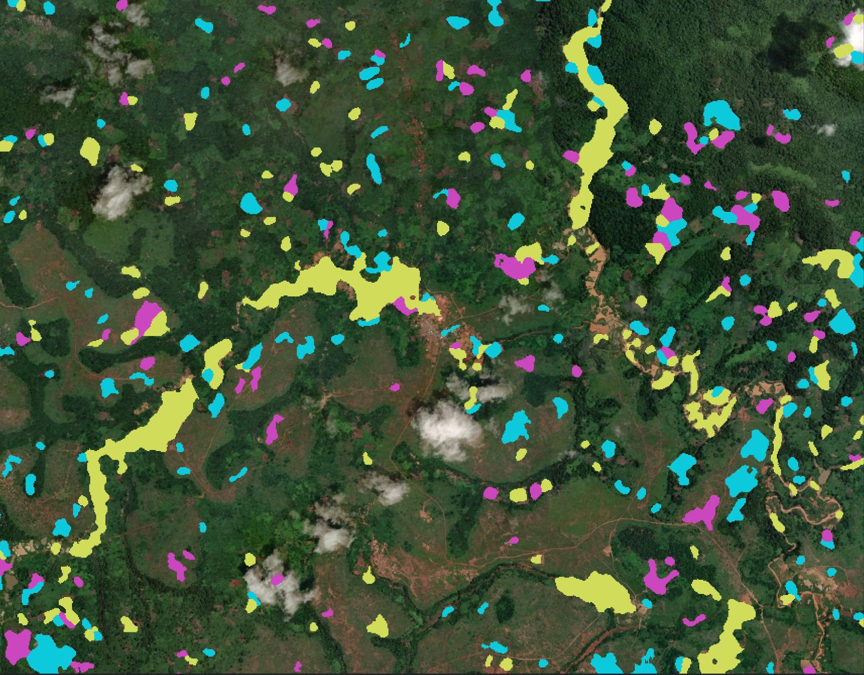
Vegetation Disturbance Occurrence disturbances from 2023 to 2025 in an area of northern DRC, drawn on the same basemap. Magnitude was thresholded and patches smaller than 7 pixels were removed. Color shows the year of disturbance (Yellow = 2023, Light blue = 2024, Pink = 2025).
6. Validation and Quality Control
Use local knowledge and independent observations to validate outputs.
Recommended checks:
- Visual comparison with high-resolution imagery. The northern DRC example pairs a current ESRI Wayback basemap with thresholded Vegetation Disturbance Occurrence patches.
- Cross-comparison with fire detections where relevant.
- Spatial consistency checks (for example isolated single-pixel artifacts).
- Temporal plausibility checks (does change year align with known events).
If results are noisy, revisit compositing and masking first, then threshold tuning.
7. Common Pitfalls to Avoid
- Treating segmentation threshold as a direct disturbance threshold.
- Running the tool on short or inconsistent time series.
- Using non-comparable seasonal windows across years.
- Interpreting disturbance from one metric alone without checking year and duration.
- Skipping local validation before operational use.
8. Simple Workflow
- Define your disturbance question and monitoring period.
- Build consistent yearly composites and select index (start with NBR).
- Confirm BAP input quality (consistent seasonal window and low residual cloud contamination).
- Run with default segmentation threshold.
- Review ChgYr, ChgMag together.
- Calibrate disturbance classification thresholds using known sites.
- Validate with independent data and refine.
- Scale to full area after settings are stable.
9. User Guidelines
Based on validation outcomes, use the following quality gates before treating outputs as operational:
- Input quality gate: verify at least three yearly observations and consistent seasonal windows across years.
- Sensitivity gate: compare at least two disturbance threshold settings and document how mapped area and patch counts change.
- Plausibility gate: check sampled locations to confirm that
ChgYraligns with known event windows and mapped patches align with imagery. - Interpretation gate: report disturbance classes together with the underlying metrics used (for example
ChgMagandChgYr) and key assumptions. - Reproducibility gate: archive final parameters, AOI version, imagery date ranges, and tool version for repeat runs.
10. Limitations
- Disturbance results are sensitive to input composite quality and seasonal consistency.
- Short time series reduce reliability and can miss pre-disturbance context.
- The approach can oversimplify pixels with repeated or multi-phase disturbances.
- Classification thresholds are not universally transferable and should be recalibrated by ecosystem and index choice.